Lecture 9: Geographically weighted regression • spatialcourseOL

Geographically weighted regression

Geographically weighted regression (GWR) is an exploratory technique mainly intended to indicate where non-stationary is taking place on the map that is where locally weighted regression coefficients move away from their global values. Its basis is the concern that the fitted coefficient values of a global model, fitted to all the data, may not represent detailed local variations in the data adequately. It differs, however, in not looking for local variation in data space but by moving a weighted window over the data, estimating one set of coefficients values at every chosen fit point. The fit points are very often the points at which observations were made, but do not have to be. If the local coefficients vary in space, it can be taken as an indication of non-stationary.

The technique is fully described by Fotheringham et al. (2002) and involves first selecting a bandwidth for an isotropic spatial weights kerner, typically a Gaussian kernel with a fixed bandwidth chosen by leave-one-out cross-validation. Choise of the bandwidth can be very demanding, as n regressions must be fitted at each step. Alternative techniques are available, for example for adaptive bandwidths, but they may often be even more compute-intensive.

In Finnish, you can read the following paper: http://ojs.tsv.fi/index.php/SA/article/viewFile/8714/6405

Geographically Weighted Regression Method

The core idea of the Geographically Weighted Regression (GWR) method is that geographically proximate areas are given greater weight than areas located farther away. Consequently, only nearby areas effectively contribute to the estimation of local regression coefficients. This weighting principle is based on Tobler’s First Law of Geography, which states that things that are near each other are more similar than things that are farther apart (Tobler, 1970). Therefore, spatially close areas contain the most relevant information for estimating local regression coefficients.

The GWR model can be defined as follows (e.g., Brunsdon et al., 1998):

$y_i = \beta_0(u_i, v_i) + \sum_{k=1}^{p} \beta_k(u_i, v_i)\, x_{i,k} + \varepsilon_i$

where

$y_i$ is the observed value of the dependent variable at location $i$ ,
$x_{i,k}$ is the value of explanatory variable $k$ at location $i$ ,
$\varepsilon_i$ is the random error term,
$(u_i, v_i)$ are the spatial coordinates of observation $i$ , and
$\beta_0(u_i, v_i)$ and $\beta_k(u_i, v_i)$ are the local regression coefficients for the intercept and explanatory variable $k$ at location $i$ .

The GWR model is based on the assumption that observations closer to the target location exert a greater influence on the estimation of parameters $\beta$ than more distant observations.

Estimation of Local Regression Coefficients

The estimation of the local regression coefficients is given by:

$\hat{\boldsymbol{\beta}}(u_i, v_i) = \left[X^T W(u_i, v_i) X \right]^{-1} X^T W(u_i, v_i) Y$

where $W(u_i, v_i)$ is an $n \times n$ spatial weighting matrix whose diagonal elements represent the geographical weights for observation $i$ , and whose off-diagonal elements are zero. A separate weight matrix is computed for each observation $i$ at which local regression coefficients are estimated.

The observation weight matrix is constructed using a kernel function based on the distances between observation points. Kernel functions are generally classified as either fixed or adaptive.

In a fixed kernel, the bandwidth (distance radius) is constant, meaning that the number of neighboring observations can vary.
In an adaptive kernel, the bandwidth varies while the number of neighboring observations remains constant.

The elements of the weight matrix are defined as:

$w_{ik} = \begin{cases} 1, & \text{if } d_{ik} < r \\ 0, & \text{otherwise} \end{cases} \tag{4}$

Gaussian Kernel Function

A commonly used weighting scheme is the Gaussian kernel, which is defined as:

$w_{ij} = \exp\left(-\frac{d_{ij}^2}{2h^2}\right) \tag{5}$

where $d_{ij}$ is the distance between observation point $i$ and regression point $j$ , and $h$ is the bandwidth parameter that defines the spatial extent within which points influence the estimation of regression coefficients.

When using point coordinates $(x, y)$ , the distance between two points is computed as the Euclidean distance:

$d_{ij} = \sqrt{(x_i - x_j)^2 + (y_i - y_j)^2} \tag{6}$

Bandwidth Selection via Cross-Validation

The bandwidth parameter $h$ is estimated using cross-validation as follows:

$\Delta(h) = \sum_{i=1}^{n} \left(y_i - \hat{y}_{(i)}(h)\right)^2 \tag{7}$

where $\hat{y}_{(i)}(h)$ is the fitted value at location $(u_i, v_i)$ obtained by excluding observation $i$ from the estimation. The goal of cross-validation is to predict each observation using the remaining data and select the bandwidth $h$ such that:

$\Delta(h) = \min \Delta(h) \tag{8}$

Statistical Significance of Local Regression Coefficients

Examining local regression coefficients does not provide meaningful insight into the relationship between explanatory and dependent variables if the standard errors of the locally estimated coefficients are large. In such cases, the effect of the explanatory variable on the dependent variable is locally random.

The statistical significance of local regression coefficients can be assessed using either a Monte Carlo test or an adapted t-test. Since the Monte Carlo method is computationally intensive, this study adopts the latter approach. Testing the significance of coefficients allows identification of explanatory variables that exhibit local spatial variation.

The t-statistic for a regression coefficient is calculated as:

$t_i = \frac{\hat{\beta}_k - 0}{SE(\hat{\beta}_k)} \tag{9}$

which follows a t-distribution with $n - 1$ degrees of freedom. This test evaluates whether the estimated regression coefficients differ significantly from zero.

To determine the significance level of the t-test, Byrne et al. (2009, p. 4) propose the following adjustment:

$F_0 = \frac{\alpha}{1 + p_e - \frac{p_e}{n p}} \tag{10}$

where

$p_e$ is the number of effective parameters,
$p$ is the number of estimated parameters,
$n$ is the number of observations, and
$\alpha$ is the chosen significance level.

You can choose the significance level based on your data. Normally, it is set to $\alpha = 0.05$ or $\alpha = 0.10$ .

Idea of Geographically Weighted Regression (GWR)

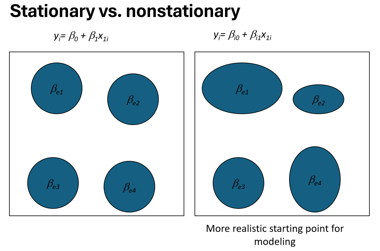
The main motivation for Geographically Weighted Regression (GWR) lies in the recognition that relationships between variables often vary across space. Traditional regression models assume spatial stationarity, meaning that the relationship between the dependent and explanatory variables is constant throughout the entire study area. This assumption is illustrated by the stationary model

$y_i = \beta_0 + \beta_1 x_{1i},$

where a single set of regression coefficients is applied uniformly to all locations.

In many spatial applications, however, this assumption is unrealistic. Social, economic, and environmental processes frequently exhibit spatial nonstationarity, meaning that the strength and form of relationships change from one location to another. This situation is illustrated in the nonstationary case, where regression parameters are allowed to vary across space:

$y_i = \beta_0(u_i, v_i) + \beta_1(u_i, v_i)x_{1i}.$

Here, $(u_i, v_i)$ denote the spatial coordinates of observation $i$ , and the regression coefficients are location-specific.

GWR addresses spatial nonstationarity by estimating a local regression model at each observation point rather than fitting a single global model. For each location, observations that are geographically closer are assigned greater weight than those farther away. As a result, locally estimated regression coefficients reflect spatial variation in the underlying relationships.

This approach allows the model to capture spatial heterogeneity that would be masked by a global regression framework. As illustrated by the figure, the stationary model assumes uniform effects across space, whereas the GWR framework provides a more realistic starting point for spatial modeling by allowing regression coefficients to vary in magnitude and spatial extent.

Geographically Weighted Regression

Example from a report: Itärata, accessibility, and socio‑economic development in Eastern Finland

In this example, we replicate an analysis from a research report that examined the relationship between accessibility and socio‑economic development in a situation where the implementation of the Eastern Rail Line (Itärata) has altered the accessibility of regions in Eastern Finland. The starting point of the study was to assess whether the development of this rail connection would improve the accessibility of Eastern Finnish regions and to examine how changes in accessibility would more broadly shape the region’s socio‑economic development. In this example, we reproduce the analysis from the report in which population change in postal code areas between 2015 and 2023 was explained by travel time to Helsinki‑Vantaa Airport. The report can be found here:

https://erepo.uef.fi/items/d186c78d-4aa9-4162-9590-1d89775bc595

Required packages

library(dplyr)
library(purrr)
library(sf)
library(GWmodel)
library(spdep)
library(ggplot2)
library(ggpubr)

Data management and description

1. Reading spatial data from the package extdata

We begin by reading the GeoPackage file that is shipped with the spatialcourseOL R package. The file is located in the package’s inst/extdata/ directory, which makes it portable across systems.

paavo_matkat <- sf::st_read(
  system.file("extdata", "paavo_matkat_ajat.gpkg",
              package = "spatialcourseOL"),
  layer = "paavo_matkat")

## Reading layer `paavo_matkat' from data source 
##   `/home/runner/work/_temp/Library/spatialcourseOL/extdata/paavo_matkat_ajat.gpkg' 
##   using driver `GPKG'
## Simple feature collection with 1305 features and 160 fields
## Geometry type: MULTIPOLYGON
## Dimension:     XY
## Bounding box:  xmin: 266300.6 ymin: 6632299 xmax: 732907.7 ymax: 7266655
## Projected CRS: ETRS89 / TM35FIN(E,N)

2. Create a working copy of the dataset

To keep the original object intact, we create a new working copy of the spatial data.

paav3<-paavo_matkat

3. Subset the data

Next, we remove extreme population change values.

Only postal code areas where population change between 2016–2024 is between −50% and +50% are retained.

paav44<-subset(paav3, muutos1624vaki<50 & muutos1624vaki>-50)

4. Correlation analysis

We examine the relationship between:

population change (muutos1624vaki)
travel time to Helsinki–Vantaa Airport (matka_aika_nyk)

Pearson’s correlation coefficient is used.

cor.test(paav44$muutos1624vaki, paav44$matka_aika_nyk)

## 
##  Pearson's product-moment correlation
## 
## data:  paav44$muutos1624vaki and paav44$matka_aika_nyk
## t = -20.017, df = 1278, p-value < 2.2e-16
## alternative hypothesis: true correlation is not equal to 0
## 95 percent confidence interval:
##  -0.5291909 -0.4457042
## sample estimates:
##       cor 
## -0.488565

5. Visualizing the relationship

Next we visualize the relationship between accessibility and population change using a scatter plot. The figure includes:

Individual observations
A LOESS smoother (non-linear trend)
A linear regression line
The Pearson correlation coefficient

ggplot(paav44, aes(matka_aika_nyk, muutos1624vaki)) +
  geom_point(alpha = 0.7, color = "#2C7FB8") +
  geom_smooth(method = "loess", se = TRUE, color = "gold2", size = 1.3 , alpha=0.15) + 
  geom_smooth(method = "lm", se = F, color = "chocolate4", size = 1.2) + # linear fit
  labs(
    x = "Travel time to airport (min)",
    y = "Population change  (%)",
    title = "Population change 2015-2023",
    subtitle = "") +
  theme_classic(base_size = 16) +
  scale_x_continuous(breaks = seq(0, 1000, by = 100)) +
  scale_y_continuous(breaks = seq(-50, 50, by = 10)) +
  ggpubr::stat_cor(
    method = "pearson",       # or "spearman"
    label.x = 0.05,           # starting x for label
    label.y = Inf,            # place at top; you can use a numeric y
    vjust = 1.2,              # tweak vertical positioning
    size = 6)  # 0, 10, 20, ...

## Warning: Using `size` aesthetic for lines was deprecated in ggplot2 3.4.0.
## ℹ Please use `linewidth` instead.
## This warning is displayed once per session.
## Call `lifecycle::last_lifecycle_warnings()` to see where this warning was
## generated.

## `geom_smooth()` using formula = 'y ~ x'
## `geom_smooth()` using formula = 'y ~ x'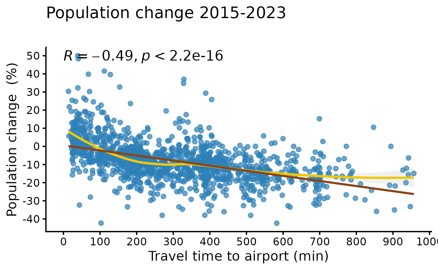

Geographically Weighted Regression (GWR): Itärata scenario

This section applies a Geographically Weighted Regression (GWR) model to analyse how accessibility (travel time) relates to population change, and how the Itärata scenario modifies this relationship at the national level.

0. Data preparation and sanity checks

We begin by preparing the spatial dataset for GWR analysis.

Only observations with valid values for:

population change (muutos1624vaki)
current travel time (matka_aika_nyk)
Itärata travel time scenario (matka_aika_itarata)

are retained.

regions_clean <- paav3 %>%
  filter(is.finite(muutos1624vaki),                # outcome used in your GWR (jobs development)
         is.finite(matka_aika_nyk),        # baseline accessibility
         is.finite(matka_aika_itarata))  # Itärata scenario accessibility

To avoid potential spatial issues, geometry validity is ensured.

regions_clean <- sf::st_make_valid(regions_clean)

The GWmodel package requires data in Spatial format, so the object is converted accordingly.

regions_sp <- as(regions_clean, "Spatial")

1. Fitting a GWR model (baseline accessibility)

Next, we fit a GWR model where population change is explained by baseline travel time to the airport.

An adaptive bandwidth approach is used, meaning that each local regression uses a fixed number of nearest neighbours.

Bandwidth selection (AICc)

bw <- bw.gwr(
  formula = muutos1624vaki ~ matka_aika_nyk,
  data    = regions_sp,
  approach= "AICc",
  kernel  = "gaussian",
  adaptive= TRUE)

## Adaptive bandwidth (number of nearest neighbours): 812 AICc value: 13077.16 
## Adaptive bandwidth (number of nearest neighbours): 510 AICc value: 13065.23 
## Adaptive bandwidth (number of nearest neighbours): 321 AICc value: 13060.06 
## Adaptive bandwidth (number of nearest neighbours): 207 AICc value: 13057.99 
## Adaptive bandwidth (number of nearest neighbours): 133 AICc value: 13053.22 
## Adaptive bandwidth (number of nearest neighbours): 91 AICc value: 13046.9 
## Adaptive bandwidth (number of nearest neighbours): 61 AICc value: 13035.18 
## Adaptive bandwidth (number of nearest neighbours): 46 AICc value: 13030.11 
## Adaptive bandwidth (number of nearest neighbours): 33 AICc value: 13025.47 
## Adaptive bandwidth (number of nearest neighbours): 29 AICc value: 13027.77 
## Adaptive bandwidth (number of nearest neighbours): 39 AICc value: 13024.77 
## Adaptive bandwidth (number of nearest neighbours): 39 AICc value: 13024.77

Fit the GWR model

gwr_model <- gwr.basic(
  formula = muutos1624vaki ~ matka_aika_nyk,
  data    = regions_sp,
  bw      = bw,
  kernel  = "gaussian",
  adaptive= TRUE)

2. Extracting local regression coefficients

From the fitted GWR model, we extract the local intercepts and slopes. These represent spatially varying relationships between accessibility and population change.

b0_local <- gwr_model$SDF$Intercept
b1_local <- gwr_model$SDF$matka_aika_nyk
summary(b1_local)

##      Min.   1st Qu.    Median      Mean   3rd Qu.      Max. 
## -0.207256 -0.073696 -0.034034  0.002327 -0.015446  2.013697

The extracted coefficients are attached back to the sf object, preserving row alignment.

regions_clean <- regions_clean %>%
  mutate(
    b0_local = b0_local,
    b1_local = b1_local)

3. Predictions and Itärata impact assessment

Using the local coefficients, we compute:

predicted population change under the baseline situation
predicted population change under the Itärata scenario
the estimated impact of Itärata

regions_clean <- regions_clean %>%
  mutate(
    x_base    = matka_aika_nyk,
    x_itarata = matka_aika_itarata,
    dx        = x_itarata - x_base,
    
    # Predictions
    yhat_base    = b0_local + b1_local * x_base,
    yhat_itarata = b0_local + b1_local * x_itarata,
    
    # Impact (Itärata - baseline) == slope * delta accessibility
    impact_itarata = yhat_itarata - yhat_base,       # same as b1_local * dx
    impact_component = b1_local * dx                  # explicitly show the contribution
  )

4. Quick diagnostics

To understand the distribution of estimated impacts, basic descriptive statistics are examined.

summary(regions_clean$impact_itarata)

##    Min. 1st Qu.  Median    Mean 3rd Qu.    Max. 
## -8.9274  0.1165  0.4171  0.6650  0.8556 17.3581

quantile(regions_clean$impact_itarata, probs = c(0, .01, .05, .5, .95, .99, 1), na.rm = TRUE)

##         0%         1%         5%        50%        95%        99%       100% 
## -8.9273859 -4.6536131 -1.0479504  0.4170597  2.0815857  9.1142592 17.3580916

5. Aggregation to regional statistics (Maakunta/County level)

Finally, population impacts are aggregated to the regional (Maakunta) level.

We first compute population change including the Itärata impact.

regions_clean$muutos1624v_imp<-regions_clean$muutos1624vaki + regions_clean$impact_itarata

Absolute population change (with and without Itärata)

a<-tapply(((regions_clean$muutos1624v_imp/100)*regions_clean$vaki24), regions_clean$Maakunta, sum)
b<-tapply(((regions_clean$muutos1624vaki/100)*regions_clean$vaki24), regions_clean$Maakunta, sum)
c<-tapply(regions_clean$vaki24, regions_clean$Maakunta, sum)

Net impact of Itärata

as<-a-b;as

##   Etelä-Karjala      Etelä-Savo          Kainuu     Kymenlaakso     Päijät-Häme 
##       1143.3694        449.6060        234.4531        186.9546      -1489.7752 
## Pohjois-Karjala    Pohjois-Savo         Uusimaa 
##       2378.1333       3212.4264      -3509.5066

sum(a-b) # erotus väestössä, n TAULUKKOON

## [1] 2605.661

Relative impact (% of population)

bs<-(a-b)/c*100 
sum(a-b)/sum(regions_clean$vaki24)*100

## [1] 0.09468731

Combined results table

abs<-cbind(as, bs); abs

##                         as         bs
## Etelä-Karjala    1143.3694  0.9199577
## Etelä-Savo        449.6060  0.3497600
## Kainuu            234.4531  0.3363023
## Kymenlaakso       186.9546  0.1181373
## Päijät-Häme     -1489.7752 -0.7366700
## Pohjois-Karjala  2378.1333  1.4804486
## Pohjois-Savo     3212.4264  1.3105098
## Uusimaa         -3509.5066 -0.2110264

Mapping the estimated Itärata impact

This map visualizes the predicted impact of the Itärata scenario on population change, based on the GWR results. The effect is shown as a continuous surface, overlaid with relevant infrastructure and reference layers

ggplot(regions_clean) +
  geom_sf(aes(fill = impact_itarata), color = NA) +
  scale_fill_viridis_c(
    option = "mako",
    direction = 1,
    name = "Impact to population \nchange (%)") +
  labs(title = "Itärata (GWR)", subtitle = "") +
  theme_minimal() +
  theme(
    panel.grid.major = element_blank(),
    panel.grid.minor = element_blank(),
    axis.text = element_blank(),
    axis.title = element_blank(),
    title = element_text(size = 16, face = 'bold'),
    legend.position = c(0.12, 0.78),
    legend.title = element_text(size = 14),
    legend.text = element_text(size = 12))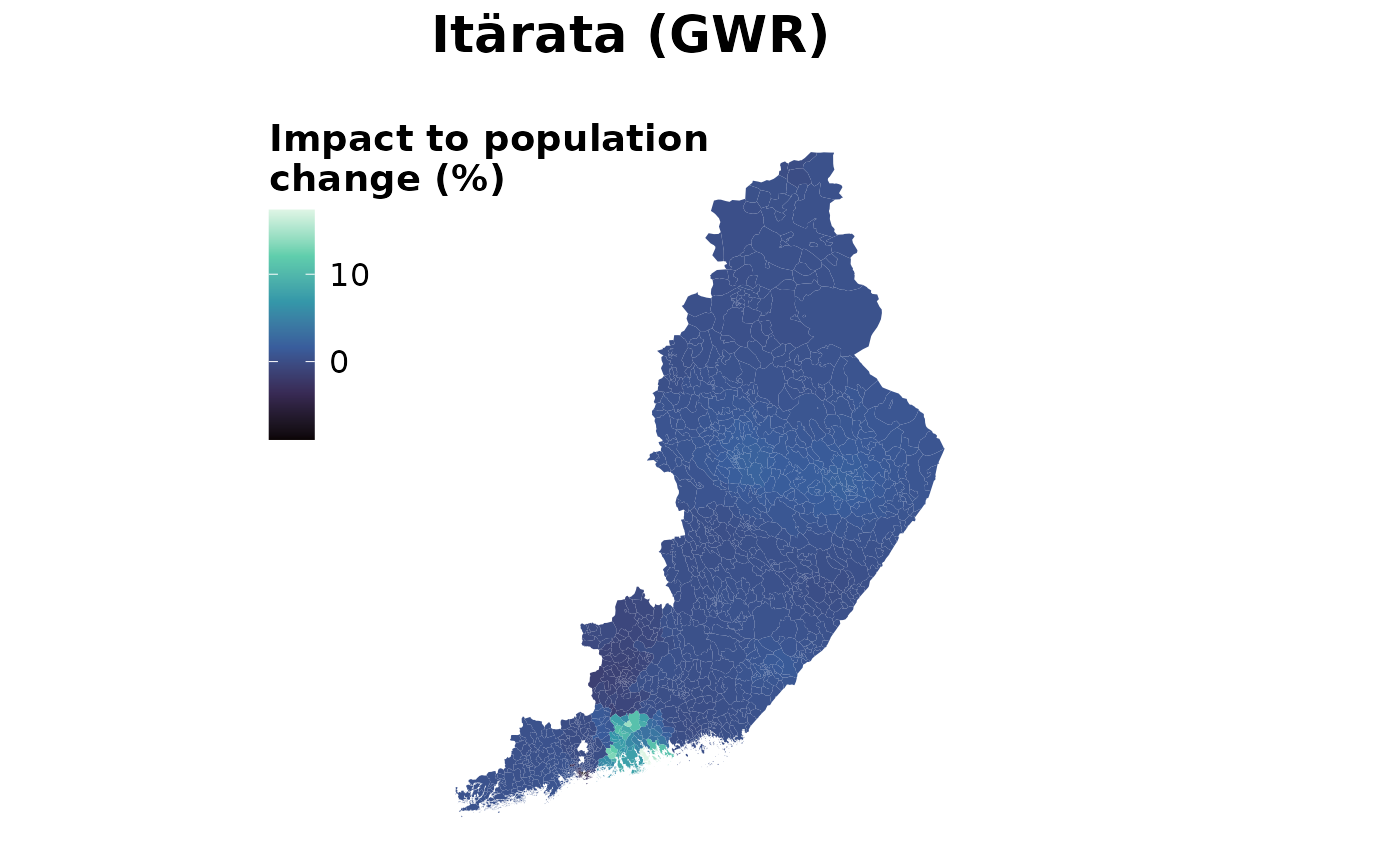

What this map shows

Each area is coloured by the estimated impact of Itärata on population change
Values are derived from local GWR coefficients
Positive values indicate areas where the rail project is predicted to mitigate population decline or support growth

Mapping local GWR regression coefficients

In addition to mapping predicted impacts, we can visualize the local regression coefficients estimated by the Geographically Weighted Regression (GWR) model. These coefficients describe how the relationship between accessibility (travel time) and population change varies across space.

In this example, we focus only on negative coefficients, which indicate areas where longer travel times are locally associated with population decline. Positive coefficients are excluded from the map to highlight spatial vulnerability more clearly.

Step 1: Mask positive coefficients

We create a new variable that keeps only negative local slope values (b1_local).

Positive coefficients are set to NA, so they will not be coloured on the map.

regions_clean$coef_neg <- ifelse(
  regions_clean$b1_local < 0,
  regions_clean$b1_local, NA)

This approach:

preserves all spatial units,
avoids changing the map extent,
makes excluded areas visually explicit.

Step 2: Plot the local coefficients

The map below shows the spatial distribution of negative GWR coefficients.

Darker colours indicate stronger negative local relationships between travel time and population change.

ggplot(regions_clean) +
  geom_sf(aes(fill = coef_neg), color = NA) +
  scale_fill_gradient2(
    low = "steelblue4",
    mid = "white",
    high = "darkred",
    midpoint = 0,
    na.value = "grey90",
    name = "Negative GWR\ncoefficients"
  ) +
  labs(
    title = "Negative local effects of travel time",
    subtitle = "Positive coefficients excluded"
  ) +
  theme_minimal()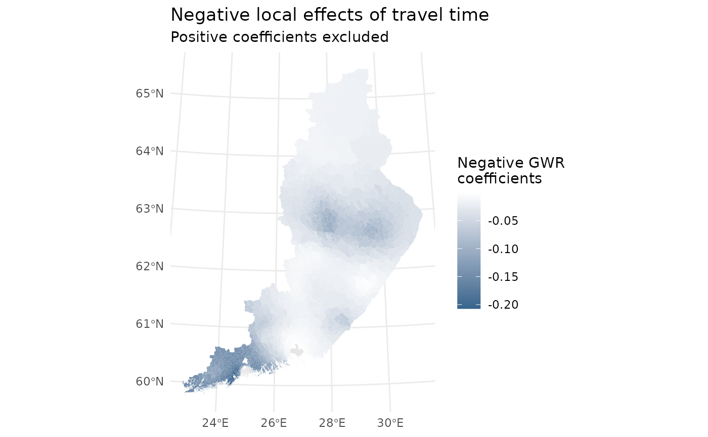

Interpretation

Darker blue areas indicate locations where increased travel time has a stronger negative association with population change.
Grey areas represent locations where the coefficient is positive or close to zero and therefore excluded from the visualization.
The spatial variation confirms non‑stationarity in the relationship between accessibility and demographic development, which is precisely what GWR is designed to reveal.

Ordinary Least Squares (OLS) benchmark model

As a point of comparison, we first estimate a global Ordinary Least Squares (OLS) regression. Unlike GWR, OLS assumes that the relationship between accessibility and population change is spatially constant, meaning the same effect applies everywhere.

In this baseline model, population change is explained by baseline travel time only, without any spatial weighting.

Fitting the OLS model

# Global OLS model without spatial weighting
ols_model <- lm(
  muutos1624vaki ~ x_base,
  data = regions_clean
)

summary(ols_model)

## 
## Call:
## lm(formula = muutos1624vaki ~ x_base, data = regions_clean)
## 
## Residuals:
##     Min      1Q  Median      3Q     Max 
## -103.83   -8.71   -3.12    3.48 1023.18 
## 
## Coefficients:
##              Estimate Std. Error t value Pr(>|t|)    
## (Intercept)  7.482255   1.847785   4.049 5.44e-05 ***
## x_base      -0.043145   0.005167  -8.350  < 2e-16 ***
## ---
## Signif. codes:  0 '***' 0.001 '**' 0.01 '*' 0.05 '.' 0.1 ' ' 1
## 
## Residual standard error: 36.65 on 1301 degrees of freedom
## Multiple R-squared:  0.05087,    Adjusted R-squared:  0.05014 
## F-statistic: 69.72 on 1 and 1301 DF,  p-value: < 2.2e-16

Interpretation

The estimated coefficient for x_base represents the average effect of travel time on population change across all regions.
The model does not account for spatial heterogeneity or local variation in relationships.
As such, it provides a useful benchmark against which the GWR results can be compared.

Using GWR with PAAVO (postal code area) data

1. Required packages

library(dplyr)
library(purrr)
library(sf)
library(httr)
library(data.table)
library(ows4R)

2. Downloading spatial data from Statistics Finland (WFS)

url <-list(hostname ="geo.stat.fi/geoserver/postialue/wfs",
           scheme ="https",
           query =list(service ="WFS",
                       version ="2.0.0",
                       request ="GetFeature",
                       typename ="postialue:pno_tilasto_2025",
                       outputFormat ="json"))%>%
  setattr("class","url")
request <-build_url(url)
p25 <-st_read(request)

## Reading layer `OGRGeoJSON' from data source 
##   `https://geo.stat.fi/geoserver/postialue/wfs/?service=WFS&version=2.0.0&request=GetFeature&typename=postialue%3Apno_tilasto_2025&outputFormat=json' 
##   using driver `GeoJSON'
## Simple feature collection with 3026 features and 113 fields
## Geometry type: MULTIPOLYGON
## Dimension:     XY
## Bounding box:  xmin: 83748.43 ymin: 6629044 xmax: 732907.7 ymax: 7776450
## Projected CRS: ETRS89 / TM35FIN(E,N)

url <-list(hostname ="geo.stat.fi/geoserver/postialue/wfs",
           scheme ="https",
           query =list(service ="WFS",
                       version ="2.0.0",
                       request ="GetFeature",
                       typename ="postialue:pno_tilasto_2016",
                       outputFormat ="json"))%>%
  setattr("class","url")
request <-build_url(url)
p16 <-st_read(request)

## Reading layer `OGRGeoJSON' from data source 
##   `https://geo.stat.fi/geoserver/postialue/wfs/?service=WFS&version=2.0.0&request=GetFeature&typename=postialue%3Apno_tilasto_2016&outputFormat=json' 
##   using driver `GeoJSON'
## Simple feature collection with 3036 features and 113 fields
## Geometry type: MULTIPOLYGON
## Dimension:     XY
## Bounding box:  xmin: 83748.43 ymin: 6629044 xmax: 732907.7 ymax: 7776450
## Projected CRS: ETRS89 / TM35FIN(E,N)

3. Data preparation and merging

names(p16)

##   [1] "id"         "gid"        "posti_alue" "nimi"       "namn"      
##   [6] "euref_x"    "euref_y"    "pinta_ala"  "vuosi"      "kunta"     
##  [11] "he_vakiy"   "he_naiset"  "he_miehet"  "he_kika"    "he_0_2"    
##  [16] "he_3_6"     "he_7_12"    "he_13_15"   "he_16_17"   "he_18_19"  
##  [21] "he_20_24"   "he_25_29"   "he_30_34"   "he_35_39"   "he_40_44"  
##  [26] "he_45_49"   "he_50_54"   "he_55_59"   "he_60_64"   "he_65_69"  
##  [31] "he_70_74"   "he_75_79"   "he_80_84"   "he_85_"     "ko_ika18y" 
##  [36] "ko_perus"   "ko_koul"    "ko_yliop"   "ko_ammat"   "ko_al_kork"
##  [41] "ko_yl_kork" "hr_tuy"     "hr_ktu"     "hr_mtu"     "hr_pi_tul" 
##  [46] "hr_ke_tul"  "hr_hy_tul"  "hr_ovy"     "te_taly"    "te_takk"   
##  [51] "te_as_valj" "te_nuor"    "te_eil_np"  "te_laps"    "te_plap"   
##  [56] "te_aklap"   "te_klap"    "te_teini"   "te_aik"     "te_elak"   
##  [61] "te_omis_as" "te_vuok_as" "te_muu_as"  "tr_kuty"    "tr_ktu"    
##  [66] "tr_mtu"     "tr_pi_tul"  "tr_ke_tul"  "tr_hy_tul"  "tr_ovy"    
##  [71] "ra_ke"      "ra_raky"    "ra_muut"    "ra_asrak"   "ra_asunn"  
##  [76] "ra_as_kpa"  "ra_pt_as"   "ra_kt_as"   "tp_tyopy"   "tp_alku_a" 
##  [81] "tp_jalo_bf" "tp_palv_gu" "tp_a_maat"  "tp_b_kaiv"  "tp_c_teol" 
##  [86] "tp_d_ener"  "tp_e_vesi"  "tp_f_rake"  "tp_g_kaup"  "tp_h_kulj" 
##  [91] "tp_i_majo"  "tp_j_info"  "tp_k_raho"  "tp_l_kiin"  "tp_m_erik" 
##  [96] "tp_n_hall"  "tp_o_julk"  "tp_p_koul"  "tp_q_terv"  "tp_r_taid" 
## [101] "tp_s_muup"  "tp_t_koti"  "tp_u_kans"  "tp_x_tunt"  "pt_vakiy"  
## [106] "pt_tyovy"   "pt_tyoll"   "pt_tyott"   "pt_tyovu"   "pt_0_14"   
## [111] "pt_opisk"   "pt_elakel"  "pt_muut"    "geometry"

p16data<-p16[,c(3,79)]
p16data<-as.data.frame(p16data[,1:2])
colnames(p16data)<-c("posti_alue","tyopy16")
p16data<-as.data.frame(p16data[,1:2])

p25_data <- dplyr::right_join(x = p16data, y = p25, by=c("posti_alue" = "postinumeroalue"))
p25_data$tyopy16[is.na(p25_data$tyopy16)] <- 0

4. Creating change variables and indicators

p25_data$tp_m22_16<-(p25_data$tp_tyopy-p25_data$tyopy16)
p25_data$tp_m22_16p<-((p25_data$tp_tyopy-p25_data$tyopy16)/p25_data$tyopy16)*100

p25_data$tyottom<-(p25_data$pt_tyott/p25_data$pt_tyoll)*100
p25_data$korkk<-(p25_data$ko_yl_kork/p25_data$ko_koul)*100
p25_data$alkut<-(p25_data$tp_alku_a/p25_data$tp_tyopy)*100
p25_data$elak<-(p25_data$te_elak/p25_data$te_taly)*100
p25_data$as_tih<-(p25_data$he_vakiy/(p25_data$pinta_ala/1000))

5. Data cleaning

p25_data2<-p25_data[,c(1,14,67,78,118:122)]

# remove na and inf
p25_data3<-p25_data2 %>%
  filter_all(all_vars(!is.infinite(.)))
p25_data4<-p25_data3 %>%
  filter_all(all_vars(!is.na(.)))

6. Join attribute data back to spatial data

data<-dplyr::left_join(x = p25, y = p25_data4, by=c("postinumeroalue" = "posti_alue"))
data2 <- data[!is.na(data$he_kika.y),] # if we don't remove NAs, we cannot join results

7. Spatial weights matrix (k‑nearest neighbours)

library(spdep)
data.coords<-st_centroid(st_geometry(data2), of_largest_polygon=TRUE) # Extracts the coordinates of each postcode area
p25_kn6<-knn2nb(knearneigh(data.coords,k=6,longlat = F)) # Returns a matrix with the indices of points belonging to the set of the k nearest neighbours of each other

## Warning in knearneigh(data.coords, k = 6, longlat = F): dnearneigh: longlat
## argument overrides object

p25_kn6_w<-nb2listw(p25_kn6)

8. Preparing GWR

This section demonstrates the main steps of a GWR analysis using R.

8.1 Required Libraries

We begin by loading the necessary R packages for spatial data handling, regression modeling, and visualization.

library(sf)
library(spgwr)
library(tidyverse)
library(patchwork)
library(janitor)
library(ggrepel)
library(ggplot2)
library(viridis)

8.2 Preparing Spatial Data

GWR requires spatial coordinates. We compute centroids for the spatial units and transform them to WGS84 (EPSG:4326). Variable names are standardized for consistency.

cntrd = st_centroid(data2)%>%
  st_transform(3067) %>%
  clean_names()

## Warning: st_centroid assumes attributes are constant over geometries

9. Global Linear Regression Model

As a baseline, we first fit a global ordinary least squares (OLS) model. This model assumes that relationships between variables are the same everywhere in the study area.

model_lm=lm(tyottom~ korkk+alkut+elak+as_tih+he_kika_x+ra_as_kpa_y, data=cntrd)
summary(model_lm) # look the results of the model

## 
## Call:
## lm(formula = tyottom ~ korkk + alkut + elak + as_tih + he_kika_x + 
##     ra_as_kpa_y, data = cntrd)
## 
## Residuals:
##     Min      1Q  Median      3Q     Max 
## -49.855  -5.061  -1.280   3.452  73.922 
## 
## Coefficients:
##              Estimate Std. Error t value Pr(>|t|)    
## (Intercept) 39.674072   1.935040  20.503  < 2e-16 ***
## korkk        0.412926   0.018719  22.059  < 2e-16 ***
## alkut       -0.032116   0.006403  -5.016 5.59e-07 ***
## elak         0.110485   0.014850   7.440 1.31e-13 ***
## as_tih      -3.353124   0.172852 -19.399  < 2e-16 ***
## he_kika_x   -0.170552   0.032218  -5.294 1.29e-07 ***
## ra_as_kpa_y -0.268296   0.011576 -23.177  < 2e-16 ***
## ---
## Signif. codes:  0 '***' 0.001 '**' 0.01 '*' 0.05 '.' 0.1 ' ' 1
## 
## Residual standard error: 9.472 on 2955 degrees of freedom
## Multiple R-squared:  0.3939, Adjusted R-squared:  0.3926 
## F-statistic:   320 on 6 and 2955 DF,  p-value: < 2.2e-16

The results provide a single estimate for each regression coefficient, representing average effects over space.

9.1 Short Interpretation of the Global Linear Regression Results

The global linear regression model explains approximately 39% of the variation in unemployment (R2=0.394R^2 = 0.394R2=0.394), indicating a moderate overall model fit. The model is highly significant overall (F-test, p<0.001p < 0.001p<0.001).

All explanatory variables are statistically significant, suggesting that they contribute meaningfully to explaining spatial variation in unemployment. A higher share of highly educated residents (korkk) and pensioners (elak) is associated with higher unemployment, whereas a higher share of employment in primary industries (alkut), higher housing density (as_tih), higher average age of population (he_kika_x), and larger average dwelling size (ra_as_kpa_y) is associated with lower unemployment.

The negative effects of housing density and average dwelling size are particularly strong, suggesting that more urbanized and higher-quality housing areas tend to experience lower unemployment levels. However, as this is a global model, the estimated coefficients represent average effects over the entire study area and do not capture potential spatial variation in relationships. Spatial patterns in residuals may therefore indicate remaining local heterogeneity, providing justification for applying a Geographically Weighted Regression (GWR) model.

9.2 Mapping Residuals of the Global Model

To examine whether spatial patterns remain unexplained, we extract model residuals and visualize them on a map.

# save residuals for plotting
data2$resid<-model_lm$residuals # create a new variable resid

# create a map from the residuals
ggplot(data2) +
  geom_sf(aes(fill=resid), color=NA) +
  scale_fill_viridis()+
  labs(title = "Residuals",
       fill="Value") +
  theme(legend.position = "left")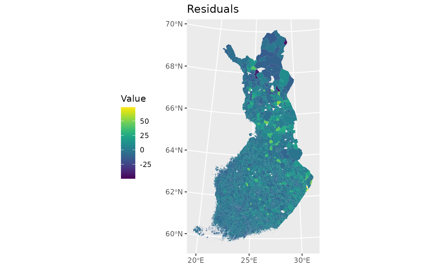

Spatial clustering in residuals may indicate spatial nonstationarity, motivating the use of GWR.

10. Converting Data for GWR

The spgwr package requires input data in the SpatialPointsDataFrame format. We therefore convert the centroid data accordingly.

cntrd.sp <- as(cntrd, "Spatial")

11. Selecting the Bandwidth

A crucial step in GWR is selecting an appropriate bandwidth, which determines how far spatial influence extends. The bandwidth is chosen using cross-validation.

# Let's analyse bandwidht
?gwr.sel
cntrd.bw=gwr.sel(tyottom~ korkk+alkut+elak+as_tih+he_kika_x+ra_as_kpa_y, data=cntrd.sp)

## Bandwidth: 490085.9 CV score: 263696.7 
## Bandwidth: 792183.9 CV score: 267669.2 
## Bandwidth: 303379 CV score: 255436.8 
## Bandwidth: 187987.8 CV score: 243369.9 
## Bandwidth: 116672.2 CV score: 230851.8 
## Bandwidth: 72596.66 CV score: 219292.2 
## Bandwidth: 45356.5 CV score: 222166.7 
## Bandwidth: 69207.22 CV score: 218475.7 
## Bandwidth: 62609.31 CV score: 217171 
## Bandwidth: 56019.32 CV score: 217151 
## Bandwidth: 59211.42 CV score: 216872.5 
## Bandwidth: 59257.14 CV score: 216873 
## Bandwidth: 59038.79 CV score: 216871.5 
## Bandwidth: 59023.84 CV score: 216871.5 
## Bandwidth: 59024.96 CV score: 216871.5 
## Bandwidth: 59025.02 CV score: 216871.5 
## Bandwidth: 59025.02 CV score: 216871.5 
## Bandwidth: 59025.01 CV score: 216871.5 
## Bandwidth: 59025.02 CV score: 216871.5 
## Bandwidth: 59025.02 CV score: 216871.5

cntrd.bw

## [1] 59025.02

The selected bandwidth defines the spatial scale at which local regressions are estimated.

What gwr.sel() is doing

gwr.sel() chooses the optimal spatial bandwidth by minimizing the cross‑validation (CV) score. During the search, R tries different bandwidth values and reports:

Bandwidth: X   CV score: Y

The algorithm keeps shrinking and adjusting the bandwidth until it finds the value that produces the lowest CV score, which measures prediction error. From your output:

Bandwidth: 59025.02 CV score: 216871.5

This is the optimal bandwidth selected for your GWR model.

The optimal GWR bandwidth selected by cross‑validation is approximately 59 km, indicating that local unemployment relationships are best estimated using information from nearby areas within this spatial range. Observations closer than 59 km exert a stronger influence on parameter estimates, while more distant observations contribute less.

12. Running the GWR Model

Using the selected bandwidth, we estimate the GWR model. Each observation receives its own set of locally weighted regression coefficients.

cntrd.gwr=gwr(tyottom~ korkk+alkut+elak+as_tih+he_kika_x+ra_as_kpa_y, data=cntrd.sp, bandwidth=cntrd.bw, hatmatrix=TRUE)
cntrd.gwr

## Call:
## gwr(formula = tyottom ~ korkk + alkut + elak + as_tih + he_kika_x + 
##     ra_as_kpa_y, data = cntrd.sp, bandwidth = cntrd.bw, hatmatrix = TRUE)
## Kernel function: gwr.Gauss 
## Fixed bandwidth: 59025.02 
## Summary of GWR coefficient estimates at data points:
##                     Min.     1st Qu.      Median     3rd Qu.        Max.
## X.Intercept. -1.3543e+01  3.0569e+01  3.7490e+01  4.4025e+01  1.0006e+02
## korkk        -1.6766e-01  2.4223e-01  3.7448e-01  5.0917e-01  1.2148e+00
## alkut        -7.2398e-01 -4.5968e-02 -9.0369e-03  4.8750e-02  9.1784e-02
## elak         -1.3149e-01 -4.3312e-03  4.0782e-02  1.0503e-01  6.5159e-01
## as_tih       -2.0046e+04 -5.4778e+00 -3.4037e+00 -2.4317e+00 -5.4232e-01
## he_kika_x    -1.4333e+00 -2.5666e-01 -1.1982e-01 -1.1343e-02  1.0090e+00
## ra_as_kpa_y  -5.5779e-01 -2.6685e-01 -2.4223e-01 -2.0048e-01  3.4253e-01
##               Global
## X.Intercept. 39.6741
## korkk         0.4129
## alkut        -0.0321
## elak          0.1105
## as_tih       -3.3531
## he_kika_x    -0.1706
## ra_as_kpa_y  -0.2683
## Number of data points: 2962 
## Effective number of parameters (residual: 2traceS - traceS'S): 154.0256 
## Effective degrees of freedom (residual: 2traceS - traceS'S): 2807.974 
## Sigma (residual: 2traceS - traceS'S): 7.605362 
## Effective number of parameters (model: traceS): 111.1774 
## Effective degrees of freedom (model: traceS): 2850.823 
## Sigma (model: traceS): 7.547991 
## Sigma (ML): 7.404981 
## AICc (GWR p. 61, eq 2.33; p. 96, eq. 4.21): 20499.81 
## AIC (GWR p. 96, eq. 4.22): 20377.72 
## Residual sum of squares: 162417.6 
## Quasi-global R2: 0.6286654

GWR substantially improves model fit compared to global OLS model, explaining ~63% of the variance.

This strongly indicates that the relationship between unemployment and the explanatory variables varies across space.

12.1 Interpretation of local coefficients (key insight)

The table of GWR coefficient summaries shows wide spatial variation: Example interpretations:

Educational level (korkk)

While the global effect is positive, some areas show negative or near-zero effects → Education affects unemployment differently in different regions

Primary-sector employment (alkut)

Mostly negative, but the effect weakens or reverses locally → Importance of primary industries is spatially uneven

Housing density (as_tih)

Strongly negative everywhere, but magnitude varies greatly → Urban structure matters, but not uniformly

Average age (he_kika_x)

Ranges from strongly negative to positive locally → Income reduces unemployment in some areas but not universally

These ranges in coefficients confirm spatial nonstationarity: the same variable can have different effects in different regions.

Conclusion: The GWR results demonstrate strong spatial nonstationarity in the determinants of unemployment. While the global model captures average national-level relationships, the GWR model reveals that the magnitude and, in some cases, the direction of these relationships vary considerably across space. The substantial improvement in model fit and the wide variation in local coefficients indicate that regional context plays a crucial role in shaping unemployment dynamics.

12.2 Exploring GWR Output

We inspect the structure of the GWR result object and identify where local coefficients are stored.

# Let's see the names of the model object
names(cntrd.gwr)

##  [1] "SDF"       "lhat"      "lm"        "results"   "bandwidth" "adapt"    
##  [7] "hatmatrix" "gweight"   "gTSS"      "this.call" "fp.given"  "timings"

# Here you can find the coefficients etc.
names(cntrd.gwr$SDF)

##  [1] "sum.w"              "(Intercept)"        "korkk"             
##  [4] "alkut"              "elak"               "as_tih"            
##  [7] "he_kika_x"          "ra_as_kpa_y"        "(Intercept)_se"    
## [10] "korkk_se"           "alkut_se"           "elak_se"           
## [13] "as_tih_se"          "he_kika_x_se"       "ra_as_kpa_y_se"    
## [16] "gwr.e"              "pred"               "pred.se"           
## [19] "localR2"            "(Intercept)_se_EDF" "korkk_se_EDF"      
## [22] "alkut_se_EDF"       "elak_se_EDF"        "as_tih_se_EDF"     
## [25] "he_kika_x_se_EDF"   "ra_as_kpa_y_se_EDF" "pred.se"

12.3 Extracting Local Regression Coefficients

We save selected local coefficients back into the original spatial dataset for mapping.

# save results to new variables
data2$coef_korkk<-cntrd.gwr$SDF$korkk
data2$coef_alkut<-cntrd.gwr$SDF$alkut

12.4 Mapping Local Coefficients

The spatial variation of regression coefficients is visualized using thematic maps. These maps reveal how the strength of relationships changes across space.

map1<-ggplot(data2) +
  geom_sf(aes(fill=coef_korkk), color=NA) +
  scale_fill_viridis() +
  labs(title = "Coefficients for \n high education",
       fill="Value") +
  theme(legend.position = "left")

map2<-ggplot(data2) +
  geom_sf(aes(fill=coef_alkut), color=NA) +
  scale_fill_viridis()+
  labs(title = "Coefficients for \n primary industries ",
       fill="Value") +
  theme(legend.position = "left")

map1 + map2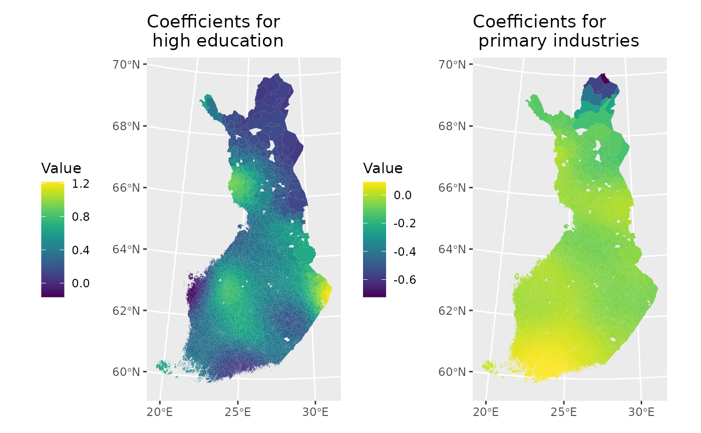

The maps show clear spatial variation in the effects of high education and primary industries on unemployment, confirming strong spatial nonstationarity. The effect of high education is positive in most parts of Finland but varies considerably in magnitude, with the strongest effects in southern and eastern regions and weaker or near-zero effects in the north. In contrast, employment in primary industries generally has a negative association with unemployment, but this effect also varies spatially, being strongest in southern and western areas and weaker or even negligible in northern regions.

Overall, these results indicate that the impact of educational structure and economic base on unemployment is region-specific, and a single national-level coefficient would mask important local differences. This supports the use of GWR over a global regression approach for analysing unemployment patterns.

13. Testing Model Improvement

Finally, we test whether allowing coefficients to vary spatially significantly improves model fit compared to the global model using the LMZ F-test. This can take some time.

# test model fit
?LMZ.F3GWR.test
LMZ.F3GWR.test(cntrd.gwr)

A significant result suggests that spatial nonstationarity is present and that GWR provides a better representation of the underlying processes than the global linear model.

Summary

This workflow demonstrates the key steps in conducting a GWR analysis in R:

Fit a global regression model
Diagnose spatial nonstationarity
Select an optimal bandwidth
Estimate local regressions
Visualize spatially varying coefficients
Statistically evaluate model improvement

GWR provides valuable insights into local spatial relationships that would be obscured in traditional global models.